详细解析轻量级光线追踪引擎的实现原理,从视口构建到透视投影的完整过程
本文详细介绍光线追踪的基本原理和实现方法,以直观的方式解释光线如何与物体相交并生成图像。文章从PPM格式图像表示开始,深入讲解射线数学表达、点乘与叉乘等向量运算的几何意义,并展示了主射线、阴影射线、反射射线和折射射线如何协同工作构建逼真的3D渲染场景。
首先理解这三件事:
人的眼睛能看到东西,是因为光从物体上反射进入到人眼,根据光线可逆性,我们可以把这个过程"想象"是由于人的眼睛发出光,投射到物体上,于是物体被看见了。现在,基于这个概念,用一条直线,带有方向,来模拟人眼,就称为 ray 线吧,即射线。
数学知识:平面有两个点:O点,P点,O 点固定,P 点运动,但是 P 点的运动受到约束:$$ (P_x-O_x)^2 + (P_y-O_y)^2 = r^2 $$ 那么 P 点的运动轨迹肯定是一个平面圆。三维的立体圆也一样。
如果 ray 向空间任意方向发射光线,再假设存在一个完全透明的立体球(此时完全看不见),当 ray 线与它相交(交点为1,在表面,交点为2,穿过内部),这个时候将交点以及交点内部都涂色,是不是马上就能看见这个立体球了?只需要满足约束:$$ (P_x-O_x)^2 + (P_y-O_y)^2 + (P_z-O_z)^2 = r^2 $$ 即可。这其实就渲染出来了一个 3D 的球体。
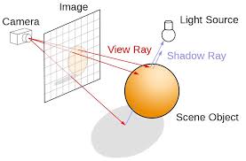
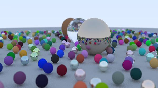
好了,理解了这个就理解了光线追踪最基本的知识,然后你就能画出如下的图了:
基础 先从最基本的来,打好基础,把框架做好。以下都是基于三维坐标进行构建的。
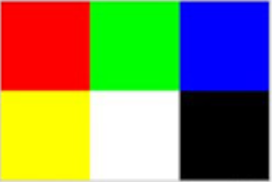
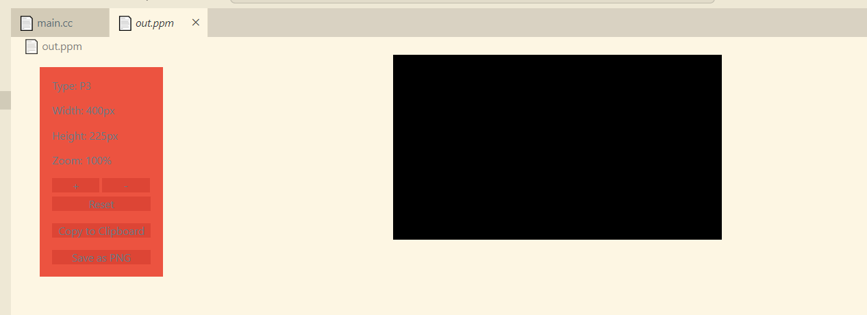
1. 如何表示图片? 这里使用 PPM 图片格式, 其最简单的内容如下:
1
2
3
4
5
6
P3 # 注释 3 2 255 255 0 0 0 255 0 0 0 255 255 255 0 255 255 255 0 0 0
所以实际图片显示如下:
2. 数学基础 射线
其中:
如果要展示具体的分量形式,可以写作:
$$ \begin{bmatrix} P_x(t) \ P_y(t) \ P_z(t) \end{bmatrix} =
涉及到向量以及矩阵,但是不需要深究,代码实现起来也不难理解。现在只需要明白几个知识点即可。
射线又可以分为:
视线射线(View Ray):
又叫做主射线,主射线是从相机/观察点(view point)发出,穿过图像平面上的每个像素,用于确定该像素"看到"的场景内容。这些射线决定了哪些物体会出现在最终渲染的图像中。
阴影射线(Shadow Ray)
相机 光源 交点 阴影射线 反射射线 折射射线 阴影射线又叫次级射线,它是从物体表面的交点发出,用于计算光照、阴影、反射和折射等效果。主要包括:
阴影射线:从交点指向光源,判断是否被遮挡
反射射线:根据反射定律计算,用于渲染镜面反射
折射射线:穿透透明物体,产生折射效果
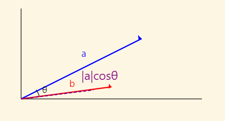
点乘
向量 a 和 b 的点乘(dot) ,表示如下:
对应的矩阵表达方式是:
*点乘的几何意义:
叉乘
对于向量 $\mathbf{a}$ 和 $\mathbf{b}$,**叉乘(cross)**可以表示为:
$$ \mathbf{a} \times \mathbf{b} = \begin{vmatrix}
展开后得到:
$$ \mathbf{a} \times \mathbf{b} = \begin{pmatrix}
叉乘的几何意义:
结果是一个向量,且垂直于 $\mathbf{a}$ 和 $\mathbf{b}$
方向遵循右手定则
模长等于 $|\mathbf{a}||\mathbf{b}|\sin\theta$
等于由两向量构成的平行四边形的面积
常用于计算法向量
用代码表示如下:
vec3.h 1 2 3 4 5 6 7 8 9 10 11 12 13 14 15 16 17 18 19 20 21 22 23 using point3 = vec3;inline double dot (const vec3& u, const vec3& v) return u.e[0 ] * v.e[0 ] + u.e[1 ] * v.e[1 ] + u.e[2 ] * v.e[2 ]; } inline vec3 cross (const vec3& u, const vec3& v) return vec3 ( u.e[1 ] * v.e[2 ] - u.e[2 ] * v.e[1 ], u.e[2 ] * v.e[0 ] - u.e[0 ] * v.e[2 ], u.e[0 ] * v.e[1 ] - u.e[1 ] * v.e[0 ] ); } inline vec3 unit_vector (const vec3& v) return v / v.length (); }
ray 射线的表达:
ray.h 1 2 3 4 5 6 7 8 9 10 11 12 13 14 15 16 17 18 19 20 21 22 23 24 #ifndef RAY_H #define RAY_H #include "vec3.h" class ray { public : ray () {} ray (const point3& origin, const vec3& direction) : orig (origin), dir (direction) {} const point3& origin () const return orig; } const vec3& direction () const return dir; } point3 at (double t) const { return orig + t*dir; } private : point3 orig; vec3 dir; }; #endif
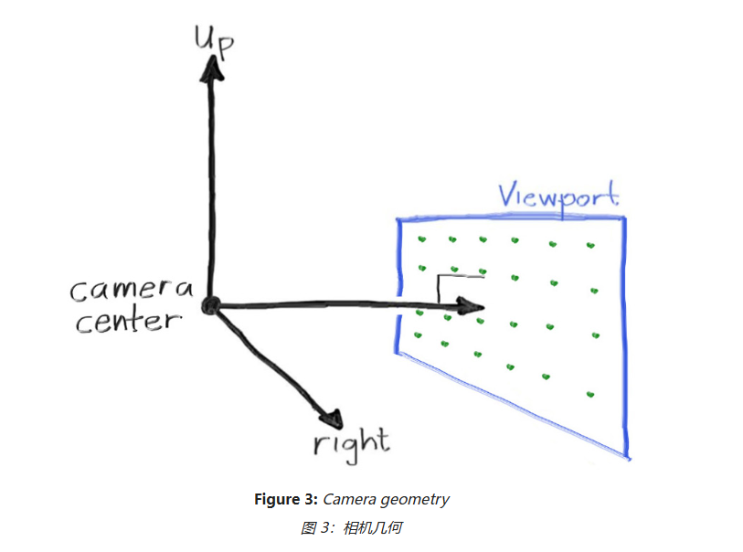
3. 空间坐标 现在假设有一个相机,它是射线的出发点,作为原点,坐标是(0,0,0)。然后还需要一个屏幕,这里我们叫做 viewport , 但是它也是虚拟的,是由像素矩阵组成的,对应着我们能看到的图像的平面。它们目前的关系如下:
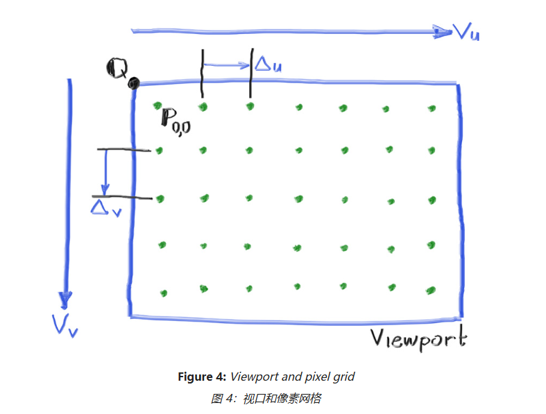
回到像素矩阵平面,其坐标如下:
这里要区分视口原点 Q,像素原点P(0,0),它们的坐标是不一样的。
现在使用代码来实现这些坐标,如下:
1 2 3 4 5 6 7 8 9 10 11 12 13 14 15 16 17 18 19 20 21 22 23 24 25 26 27 28 29 30 31 32 33 auto aspect_ratio = 16.0 / 9.0 ; int image_width = 400 ; int image_height = int (image_width / aspect_ratio); image_height = (image_height < 1 ) ? 1 : image_height; auto focal_length = 1.0 ; auto viewport_height = 2.0 ; auto viewport_width = viewport_height * (double (image_width)/image_height); auto camera_center = point3 (0 , 0 , 0 ); auto viewport_u = vec3 (viewport_width, 0 , 0 ); auto viewport_v = vec3 (0 , -viewport_height, 0 ); auto pixel_delta_u = viewport_u / image_width; auto pixel_delta_v = viewport_v / image_height; auto viewport_upper_left = camera_center - vec3 (0 , 0 , focal_length) - viewport_u/2 - viewport_v/2 ; auto pixel00_loc = viewport_upper_left + 0.5 * (pixel_delta_u + pixel_delta_v);
有了相机中心点,viewport的左上角的点,和像素的第一个点(扫描所有像素点时,从左到右,从上到下,因此左上角是起点)
1 2 3 4 5 6 7 8 9 10 11 12 13 14 15 16 17 18 19 20 for (int j = 0 ; j < image_height; j++) { for (int i = 0 ; i < image_width; i++) { auto pixel_center = pixel00_loc + (i * pixel_delta_u) + (j * pixel_delta_v); auto ray_direction = pixel_center - camera_center; ray r (camera_center, ray_direction) ; color pixel_color = ray_color (r); write_color (std::cout, pixel_color); } } color ray_color (const ray& r) { return color (0 ,0 ,0 ); }
4. 渲染 前面已经完成部分代码,以下是主代码:
1 2 3 4 5 6 7 8 9 10 11 12 13 14 15 16 17 18 19 20 21 22 23 24 25 26 27 28 29 30 31 32 33 34 35 36 37 38 39 40 41 42 43 44 45 46 47 48 49 50 51 52 53 54 #include "color.h" #include "ray.h" #include "vec3.h" #include <iostream> color ray_color (const ray& r) { return color (0 ,0 ,0 ); } int main () auto aspect_ratio = 16.0 / 9.0 ; int image_width = 400 ; int image_height = int (image_width / aspect_ratio); image_height = (image_height < 1 ) ? 1 : image_height; auto focal_length = 1.0 ; auto viewport_height = 2.0 ; auto viewport_width = viewport_height * (double (image_width)/image_height); auto camera_center = point3 (0 , 0 , 0 ); auto viewport_u = vec3 (viewport_width, 0 , 0 ); auto viewport_v = vec3 (0 , -viewport_height, 0 ); auto pixel_delta_u = viewport_u / image_width; auto pixel_delta_v = viewport_v / image_height; auto viewport_upper_left = camera_center - vec3 (0 , 0 , focal_length) - viewport_u/2 - viewport_v/2 ; auto pixel00_loc = viewport_upper_left + 0.5 * (pixel_delta_u + pixel_delta_v); std::cout << "P3\n" << image_width << " " << image_height << "\n255\n" ; for (int j = 0 ; j < image_height; j++) { std::clog << "\rScanlines remaining: " << (image_height - j) << ' ' << std::flush; for (int i = 0 ; i < image_width; i++) { auto pixel_center = pixel00_loc + (i * pixel_delta_u) + (j * pixel_delta_v); auto ray_direction = pixel_center - camera_center; ray r (camera_center, ray_direction) ; color pixel_color = ray_color (r); write_color (std::cout, pixel_color); } } std::clog << "\rDone. \n" ; }
渲染的关键部分在于,获得 ray 射线后:
1 2 3 4 5 6 7 8 9 10 11 ray r (camera_center, ray_direction) ; color pixel_color = ray_color (r); write_color (std::cout, pixel_color); color ray_color (const ray& r) { return color (0 ,0 ,0 ); }
结果如下:
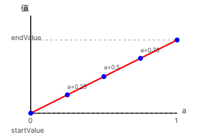
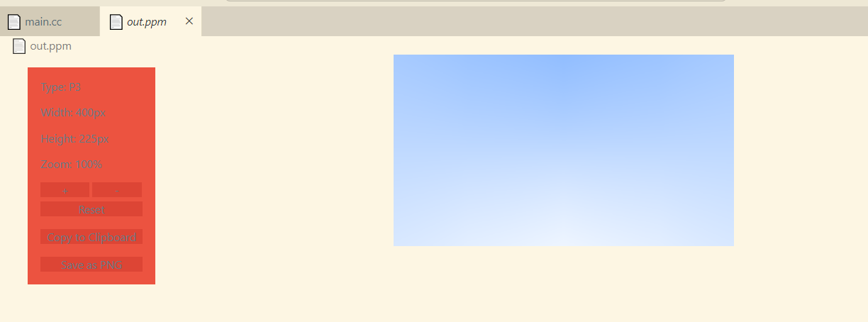
为了渲染其他颜色,需要更改 ray_color 的逻辑。这里我们想先做一个简单的渐变效果。
有一种方法叫做线性混合 或 线性插值 : $$ f(a) = (1-a) \cdot v_0 + a \cdot v_1 $$
应用到代码中是这样:
1 2 3 4 5 color ray_color (const ray& r) { vec3 unit_direction = unit_vector (r.direction ()); auto a = 0.5 *(unit_direction.y () + 1.0 ); return (1.0 -a)*color (1.0 , 1.0 , 1.0 ) + a*color (0.5 , 0.7 , 1.0 ); }
所有图片变成渐变了:
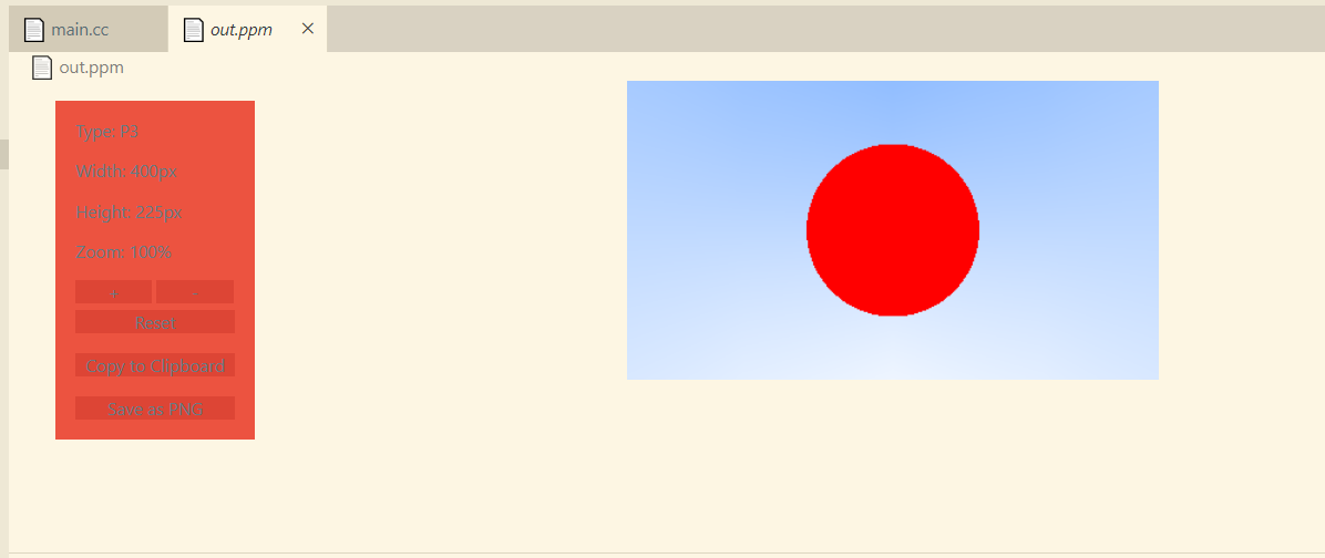
5. 渲染球体 根据前面的数学知识,我们已经知道了绘制一个想象中的球体是如何了。假设我们要在 viewport 中心处渲染处这个球体,目前球的中心点已知,ray 射线也已知,那么只剩下解方程了。
P=(x,y,z)到中心 C=(Cx,Cy,Cz) 的向量是 (C−P), 那么球的表明方程为:(C−P)⋅(C−P)=r2
求球根公式是:
1 2 3 4 5 6 7 8 9 10 11 12 13 14 15 16 17 18 19 20 21 22 23 24 25 26 bool hit_sphere (const point3& center, double radius, const ray& r) vec3 oc = center - r.origin (); auto a = dot (r.direction (), r.direction ()); auto b = -2.0 * dot (r.direction (), oc); auto c = dot (oc, oc) - radius*radius; auto discriminant = b*b - 4 *a*c; 大于或等于 0 时,说明有根,因此射线 ray 与球体相交。 return (discriminant >= 0 ); } color ray_color (const ray& r) { if (hit_sphere (point3 (0 ,0 ,-1 ), 0.5 , r)) return color (1 , 0 , 0 ); vec3 unit_direction = unit_vector (r.direction ()); auto a = 0.5 *(unit_direction.y () + 1.0 ); return (1.0 -a)*color (1.0 , 1.0 , 1.0 ) + a*color (0.5 , 0.7 , 1.0 ); }
结果如预期一样,渲染出了一个球体,从想象中透明的球体变为可见的了。
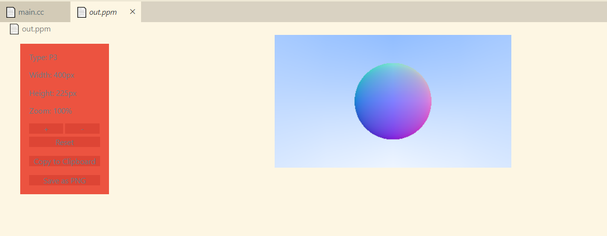
6. 球体表面法线着色 球体表面的法线即为垂直于表面的一条线,在坐标系中它位于从球心指向表面交点的方向。
刚才我们使用 ray 射线进行着色,现在使用球体表面法线进行着色。
代码如下:
1 2 3 4 5 6 7 8 9 10 11 12 13 14 15 16 17 18 19 20 21 22 23 24 25 26 27 28 29 double hit_sphere (const point3& center, double radius, const ray& r) vec3 oc = center - r.origin (); auto a = dot (r.direction (), r.direction ()); auto b = -2.0 * dot (r.direction (), oc); auto c = dot (oc, oc) - radius*radius; auto discriminant = b*b - 4 *a*c; if (discriminant < 0 ) { return -1.0 ; } else { return (-b - std::sqrt (discriminant) ) / (2.0 *a); } } color ray_color (const ray& r) { auto t = hit_sphere (point3 (0 ,0 ,-1 ), 0.5 , r); if (t > 0.0 ) { vec3 N = unit_vector (r.at (t) - vec3 (0 ,0 ,-1 )); return 0.5 *color (N.x ()+1 , N.y ()+1 , N.z ()+1 ); } vec3 unit_direction = unit_vector (r.direction ()); auto a = 0.5 *(unit_direction.y () + 1.0 ); return (1.0 -a)*color (1.0 , 1.0 , 1.0 ) + a*color (0.5 , 0.7 , 1.0 ); }
于是球体也有了渐变色:
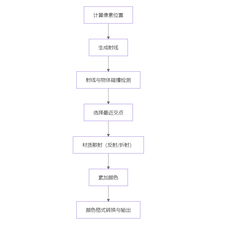
后续 用下面的示意图总结一下整个渲染流程的核心步骤:
后面还有对交点附近的点进行抗锯齿处理、表面漫反射处理、折射处理,以及根据不同材料表面的反射情况做不同的处理等等更复杂的处理,时间有限,这样就先不写了,后面有时间再继续写。有兴趣可以看参考链接。
参考链接: https://raytracing.github.io/books/RayTracingInOneWeekend.html